1. Simple Distribution Fitting
In these examples we just use our laplace approximation to fit a known posterior distribution in one and two dimensions, and see how well it reproduces the posterior.
1.1. One Dimension Beta Distribution
import jax.numpy as jnp
from jax import random
from melvin import LaplaceApproximation
import jax
import matplotlib.pylab as plt
from functools import partial

jax.config.update("jax_enable_x64", True)
WARNING:absl:No GPU/TPU found, falling back to CPU. (Set TF_CPP_MIN_LOG_LEVEL=0 and rerun for more info.)
SEED = random.PRNGKey(220)

MU = 0.3
APB = 10

ALPHA = MU * APB
BETA = (1.0 - MU) * APB
class BetaPosteriorOptimizer(LaplaceApproximation):
    param_bounds = jnp.array([[0.0, 1.0]])

    def log_prior(self, params):
        return jax.scipy.stats.beta.logpdf(x=params[0], a=ALPHA, b=BETA)

    def log_likelihood(self, params, y, y_pred):
        return 0.0

initial_params = jnp.array([0.5])

model = BetaPosteriorOptimizer(
    name="Beta Posterior Optimizer",
    initial_params=initial_params
)
print(model)
/opt/hostedtoolcache/Python/3.9.5/x64/lib/python3.9/site-packages/scipy/optimize/_minimize.py:524: RuntimeWarning: Method BFGS does not use Hessian information (hess).
  warn('Method %s does not use Hessian information (hess).' % method,
Laplace Approximation: Beta Posterior Optimizer
Base distribution: normal
Fixed Parameters: []
Fit converged successfully
Fitted Parameters:
[
  0.2500002248973315 +/- 0.15309315483089667,	 [Lower Bound = 0.0]	 [Upper Bound = 1.0]
]
MAP Posterior Prob = 1.030747930559878
x = jnp.linspace(0.0, 1.0, 100)
y = jax.scipy.stats.beta.pdf(x=x, a=ALPHA, b=BETA)
laplace_logpdf_vec = jax.vmap(model.laplace_log_posterior)
y_approx = jnp.exp(laplace_logpdf_vec(x.reshape(-1,1)).reshape(-1))
SEED, _seed = random.split(SEED)
samples = model.sample_params(prng_key=_seed, n_samples=10_000, method="simple")
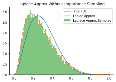
plt.plot(x,y,label="True PDF")
plt.plot(x,y_approx, label="Laplac Approx")
plt.hist(samples.reshape(-1), bins=x, density=True, label="Laplace Approx Samples", alpha=0.6)
plt.title("Laplace Approx Without Importance Sampling")
plt.legend()
plt.show()
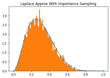
importance_samples = model.sample_params(prng_key=_seed, n_samples=10_000, method="importance")

plt.plot(x,y, label="True PDF")
plt.hist(importance_samples.reshape(-1), bins=x, density=True, label="Importance-Laplace Approx Samples")
plt.title("Laplace Approx With Importance Sampling")
plt.show()
_ = model.sample_params(prng_key=_seed, n_samples=10_000, verbose=True)
Method = simple, Perf = -0.028725638395464936
Method = importance,	 Perf = 0.010597685119911437
**Best Method = importance**
1.2. Two Dimensional: Normal / Gamma
X_MU = 2.0
X_STD = 1.0
Y_MU = 5.0
Y_SCALE = 1.0
class NormalGammaOptimizer(LaplaceApproximation):
    param_bounds = jnp.array([[jnp.nan, jnp.nan], [0, jnp.nan]])

    def log_prior(self, params):
        x_log_pdf = jax.scipy.stats.norm.logpdf(x=params[0], loc=X_MU, scale=X_STD)
        y_log_pdf = jax.scipy.stats.gamma.logpdf(x=params[1], a=Y_MU, scale=Y_SCALE)
        return x_log_pdf + y_log_pdf

    def log_likelihood(self, params, y, y_pred):
        return 0.0

initial_params = jnp.array([0.5, 0.2])

model = NormalGammaOptimizer(
    name="Normal Gamma Optimizer",
    initial_params=initial_params,
)
print(model)
/opt/hostedtoolcache/Python/3.9.5/x64/lib/python3.9/site-packages/scipy/optimize/_minimize.py:524: RuntimeWarning: Method BFGS does not use Hessian information (hess).
  warn('Method %s does not use Hessian information (hess).' % method,
Laplace Approximation: Normal Gamma Optimizer
Base distribution: normal
Fixed Parameters: []
Fit converged successfully
Fitted Parameters:
[
  2.0000026375787967 +/- 1.0,
  4.000001361417955 +/- 2.0000003403544597,	 [Lower Bound = 0.0]
]
MAP Posterior Prob = -2.5518149190767656
x = jnp.linspace(-0.5,4.5,100)
y = jnp.linspace(0.0,10.0,100)

xy = jnp.array([
    [x_i, y_i] for y_i in y for x_i in x
])

model_vec = jax.vmap(model._log_posterior, (0, None, None))
log_pdf_true = model_vec(xy, None, None).reshape(100,100)
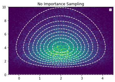
samples = model.sample_params(prng_key=_seed, n_samples=100_000, method="simple").reshape(-1, 2)
plt.contour(x, y, jnp.exp(log_pdf_true), linestyles="dashed", levels=10, lw=1, colors="white")
plt.hist2d(samples[:,0], samples[:,1], bins=(x,y))
plt.legend()
plt.title("No Importance Sampling")
plt.show()
<ipython-input-11-ff3f2b4fc57c>:1: UserWarning: The following kwargs were not used by contour: 'lw'
  plt.contour(x, y, jnp.exp(log_pdf_true), linestyles="dashed", levels=10, lw=1, colors="white")
WARNING:matplotlib.legend:No handles with labels found to put in legend.
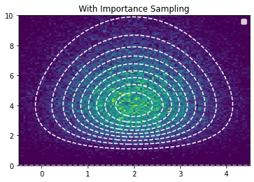
importance_samples = model.sample_params(prng_key=_seed, n_samples=100_000, method="importance").reshape(-1, 2)
plt.contour(x, y, jnp.exp(log_pdf_true), linestyles="dashed", levels=10, lw=1, colors="white")
plt.hist2d(importance_samples[:,0], importance_samples[:,1], bins=(x,y))
plt.legend()
plt.title("With Importance Sampling")
plt.show()
<ipython-input-13-bb968569afbe>:1: UserWarning: The following kwargs were not used by contour: 'lw'
  plt.contour(x, y, jnp.exp(log_pdf_true), linestyles="dashed", levels=10, lw=1, colors="white")
WARNING:matplotlib.legend:No handles with labels found to put in legend.
_ = model.sample_params(prng_key=_seed, n_samples=100_000, verbose=True)
Method = simple, Perf = -0.025580800421618033
Method = importance,	 Perf = 0.014126322603956076
**Best Method = importance**